BACKGROUND

Convolutional Neural Networks (CNN)

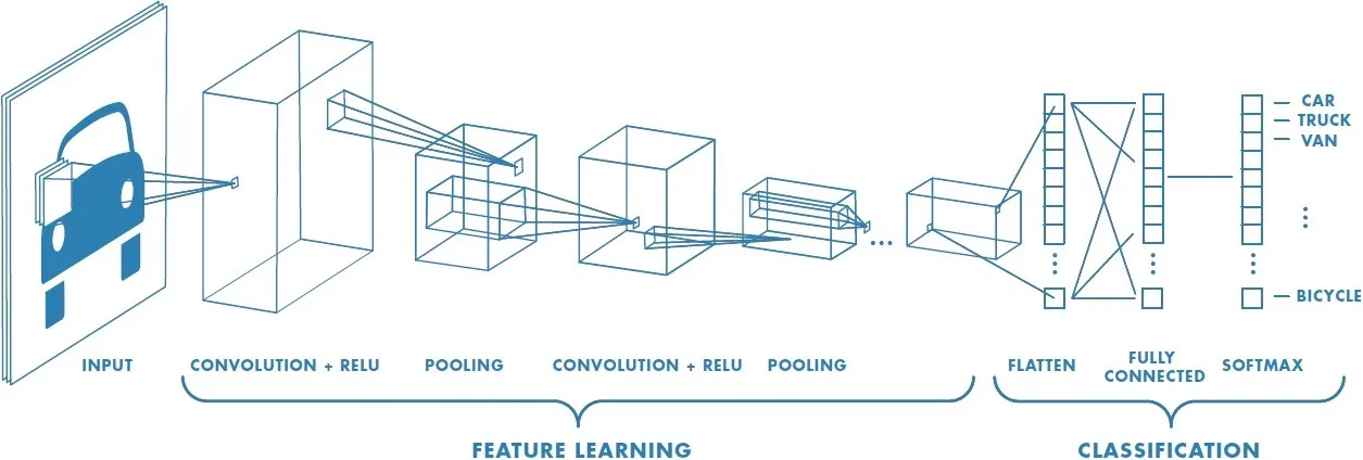
Convolutional Neural Networks (CNNs) are a powerful class of deep neural networks that have shown remarkable success in a variety of computer vision tasks, such as image classification, object detection, and segmentation. CNNs were inspired by the visual processing mechanism of the human brain and are designed to automatically learn hierarchical representations of visual features from raw data, such as images.

The key component of a CNN is the convolutional layer, which applies a set of learnable filters to the input image to extract local features. These filters slide over the entire image and perform a dot product operation with the local patch of pixels they are currently positioned over. By stacking multiple convolutional layers, the network can learn increasingly abstract and complex features, allowing it to capture high-level information such as object shapes, textures, and patterns. In addition to the convolutional layers, CNNs also typically include pooling layers to reduce the spatial dimensions of the feature maps and improve the computational efficiency of the network, and fully connected layers to perform the final classification or regression task.

Image Source

Training a CNN involves optimizing the network’s parameters using a loss function and backpropagation algorithm, similar to other types of neural networks. However, due to their larger number of parameters and deeper architectures, CNNs require large amounts of labeled data and significant computational resources for training. Overall, CNNs have revolutionized the field of computer vision and have achieved state-of-the-art performance on many benchmark datasets. They have also found applications in other domains such as natural language processing and speech recognition.

Transfer Learning

Transfer learning is a machine learning technique that involves using a pre-trained neural network to solve a new task. Instead of training a neural network from scratch, transfer learning involves taking an existing neural network that has already been trained on a large dataset and adapting it for a new task. The pre-trained neural network is typically a deep neural network that has learned to recognize complex features in images. To adapt the pre-trained network for a new task, the final layers of the network are typically replaced with new layers that are specific to the new task. These new layers are then trained on a smaller dataset that is specific to the new task. This approach allows for the transfer of knowledge from the pre-trained network, which has learned to recognize general features, to the new task, which may require more specialized features. Some examples of popular CNN architectures used in transfer learning are Visual Geometry Group (VGG) models, Residual Neural Networks (ResNet) models and Inception.

OBJECTIVES

This project focuses on training a Convolutional Neural Network (CNN) for a supervised classification task, specifically for predicting the presence of pulmonary edema and pleural effusion in chest radiographs. The project is a series of experiments to formulate a pipeline based on deep learning best practices, to achieve the best performing model for this multi-label classification task. The first experiment involved determining the appropriate application of transfer learning to chest radiograph image data. The second experiment involved testing different formulations of the problem statement to achieve the best performing model. Separated binary label classifiers, a multi-label classifier and a multi-class classifier were all trained and evaluated using label prediction accuracy and the AUC (Area Under the Curve) of the ROC (Receiver Operating Characteristic) curve which is a measure of the model’s discriminability.

METHODS

Experiment I: Determining a Model Training Pipeline

The decision of when to unfreeze layers in a pre-trained neural network depends on several factors, such as the size and similarity of the new dataset to the original dataset, the complexity of the new task, and the performance of the model on the new task. The following decision matrix outlines the appropriate use of transfer learning to obtain the best performance.

Image Source

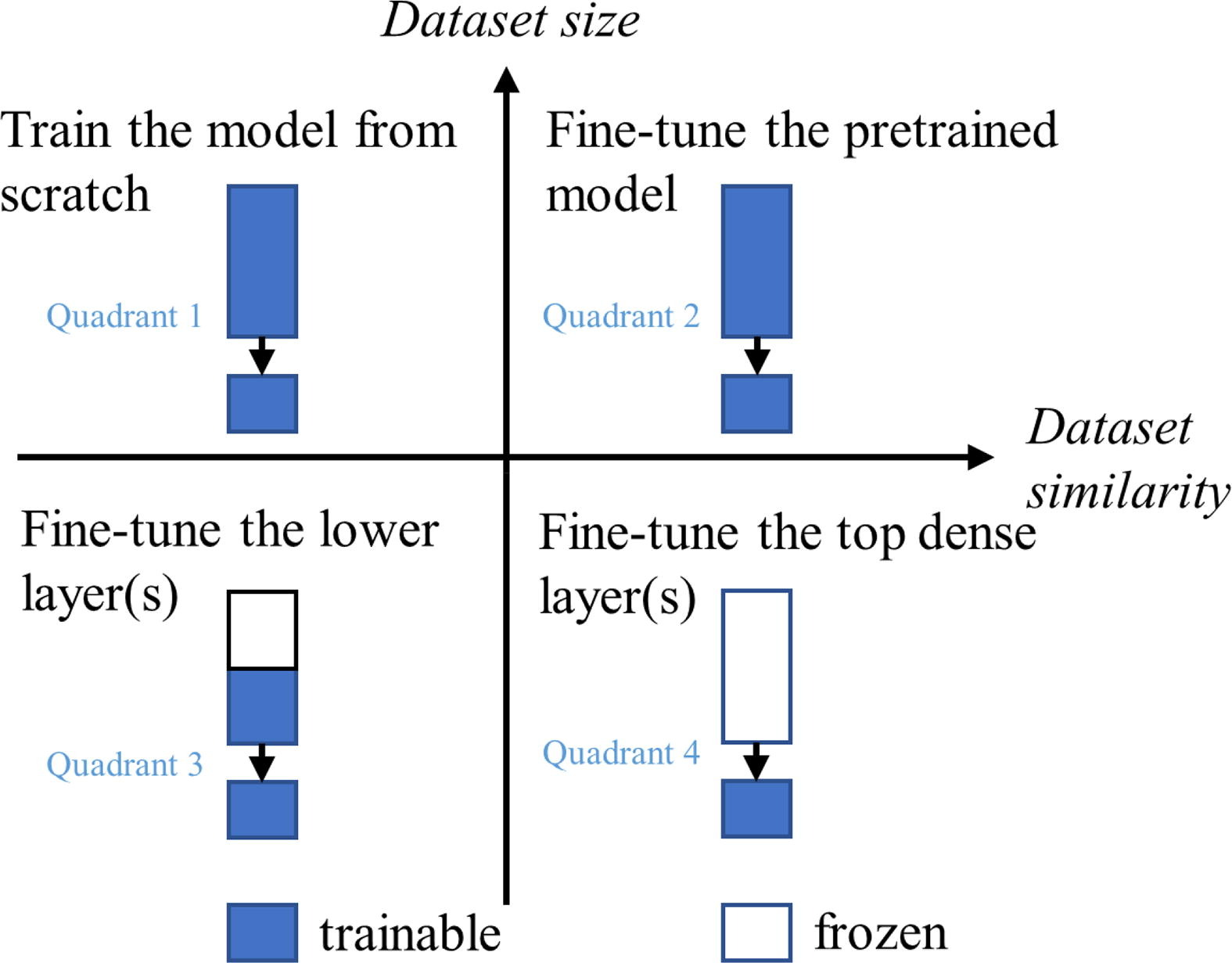
In this instance, the ImageNet dataset, on which the transfer learning architecture is pre-trained on, consists of over 14 million images, which have been annotated with object labels and bounding boxes. The chest radiograph image data used in this project is dissimilar enough to the ImageNet dataset to warrant an investigation into whether layers with pre-trained weights should be unfrozen in the training process. This experiment was conducted partly during Quarter 1, and extended for its specific application for this quarter’s project. During Quarter 1, I trained a CNN regression model on similar chest radiograph image data with continuous BNPP serum biomarker labels from a dataset compiled at UCSD Health. Initially, I left all 566 layers in the ResNet152 architecture frozen but quickly realized that due to the huge imbalance in number of trainable to untrainable parameters, the model simply wasn’t learning. Therefore, I decided to explore unfreezing certain layers iteratively in the following schedule, and observed the following:

Epochs	Unfrozen Layers	MAE	Accuracy	ROC Score
0 - 35	Last 3 Layers only	0.6608	65.5%	0.661
35 - 50	Conv 5 Block 3	0.5818	72.2%	0.763
50 - 70	Conv 5 (All Blocks)	0.5398	75.5%	0.805
70 - 80	Conv 4 (Last 3 Blocks) + Conv Layer 5	0.5472	74.6%	0.801

The major observation from this experiment was that unfreezing further layers in the architecture allows the model to better fit to the new dataset, up until a certain point where it would begin to overfit as seen when Convolution Layer 4 was also unfrozen for learning.

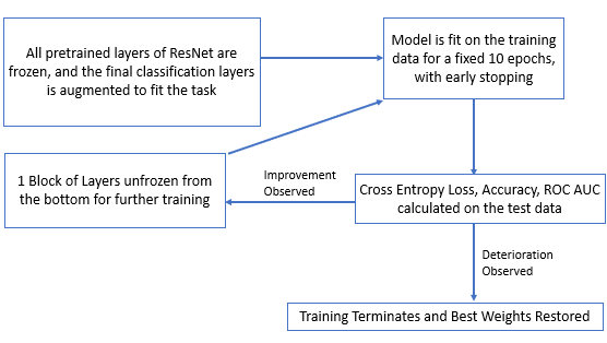
The Model Training Pipeline shown in the figure was adapted from the Quarter 1 experiment with a few changes. Since the task at hand for this project is a classification task with binary labels as opposed to regression with a continuous target, the ResNet152 architecture tended to fit more quickly to the training data, despite the larger dataset being used for this project. Therefore, each setting of the model was trained for a shorter duration of 10 epochs with early stopping, and only one block of layers were unfrozen between settings as opposed to multiple blocks of layers.

Experiment II: Determining the best model for the multi-label classification task

Three approaches to implementing this multi-label classification task will be explored in this experiment, each with their own advantages and disadvantages. The following figure is a representation of the respective model architectures:

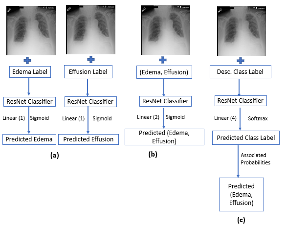
Model (a) describes a set of binary label classifiers. In this method, two separate ResNet152 architectures are trained, one using the Pulmonary Edema label and the other, the Pleural Effusion label. The final layer is augmented to a fully connected linear layer, with one output activated by a sigmoid function.

Model (b) describes a multi-label classifier. In this method, one ResNet152 architecture is trained with both labels as the input. The final layer is augmented to a fully connected linear layer, with two outputs activated by a sigmoid function, corresponding to the pulmonary edema and pleural effusion labels.

Model (c) describes a multi-class classifier. The use of a multi-class classifier for a multi-label classification task is counterintuitive. However, when considering that pulmonary edema and pleural effusion are conditions that often present together in patients, the dataset of ~34,000 is skewed towards cases with the labels (0, 0) or (1, 1).

It would be worthwhile to investigate a training method where the loss calculated during training is weighted by a proportion inverse to its label representation in the dataset. Therefore, this class imbalance is addressed by reframing the multi-label classification task as a multi-class classification task where the array of labels are collapsed as: {(0, 0): 0, (0, 1): 1, (1, 0): 2, (1, 1): 3}, into 4 classes. For this classifier, the final layer is augmented to a fully connected linear layer, with four outputs activated by a softmax function, with each output corresponding to prediction confidence probability of each class. Once the model provides its prediction on the test data, the four outputs are concatenated using those probabilities in the following manner:

• Prediction for Presence of Pulmonary Edema: (0 * P(0)) + (0 * P(1)) + (1 * P(2)) + (1 * P(3))
• Prediction for Presence of Pulmonary Edema: (0 * P(0)) + (1 * P(1)) + (0 * P(2)) + (1 * P(3))

RESULTS

The following figures and table show the results of the best model obtained for the methods (a), (b) and (c). The first set of figures are the confusion matrices of the model predictions for the Pulmonary Edema Label on an unseen test set (n = 3371). A confusion matrix visualizes the number of true positives, false positives, false negatives and true negatives. The raw outputs of each model were converted to binary predictions at the threshold 0.5:

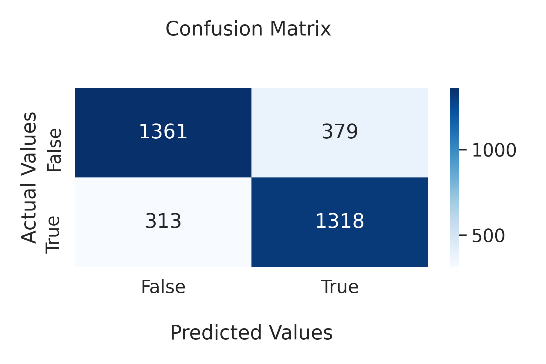
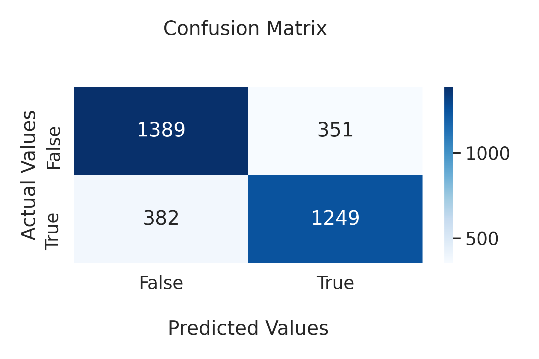
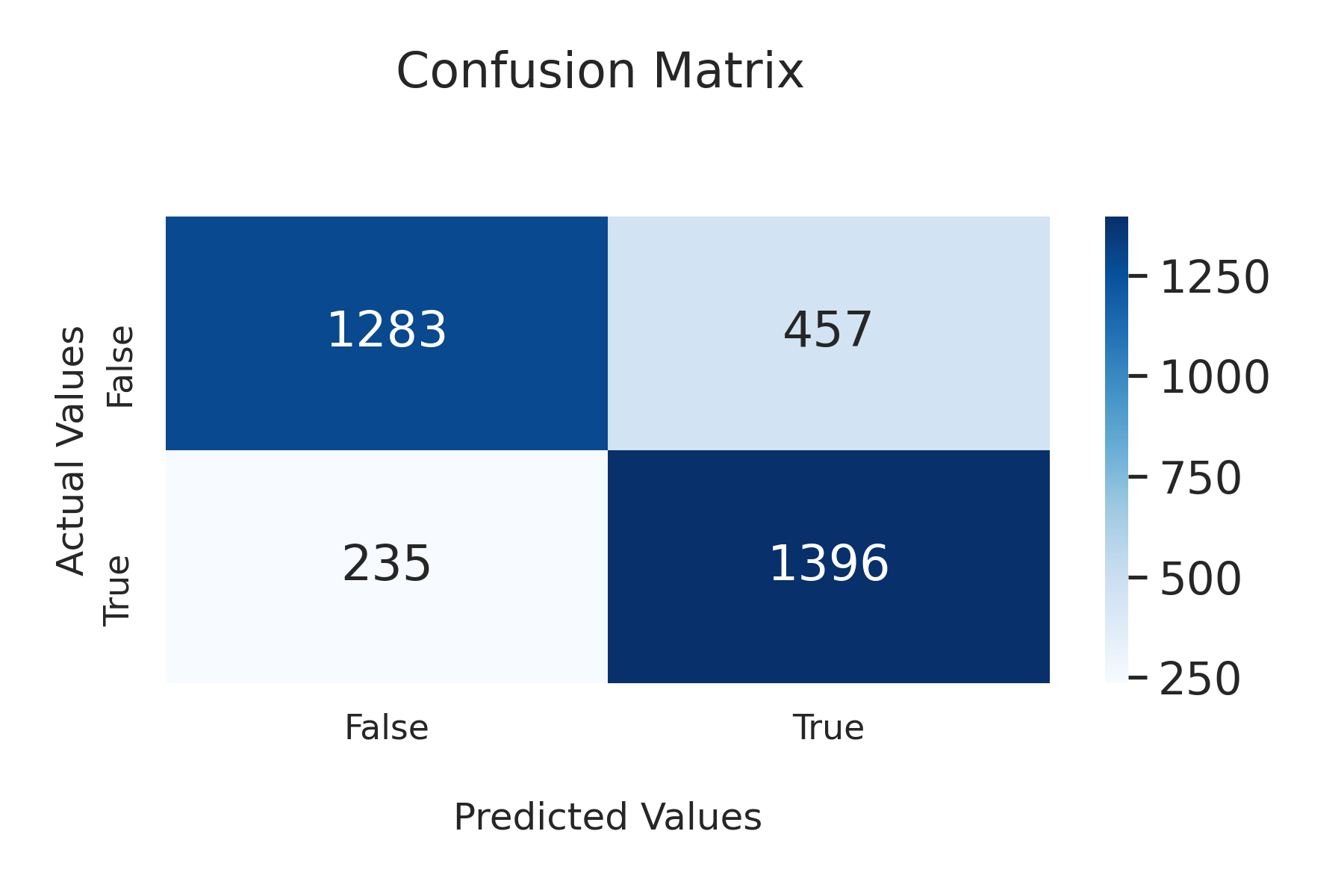
(From left to right: Single Label Classifier, Multi-label Classifier, Multi-class Classifier)

The following two figures are a summary comparison of the models’ discriminability, i.e the ability of the classifier to distinguish between the binary labels, as measured using the area under the ROC curve:

Finally, these last two figures are a comparison of the models’ performance on accuracy across both labels and their training time:

CONCLUSION

In this project, I investigated the effectiveness of progressively unfreezing blocks of layers in the large ResNet152 architecture for a binary-label classification task involving pulmonary edema and pleural effusion, and found that this technique led to a speed-up in model convergence before overfitting occurred, which improved the overall efficiency of the model. I also compared the performance of multiclass and multilabel classifiers for this task, and found that the multiclass classifier was a more efficient method when considering training time, with little to no tradeoff in overall prediction accuracy or model discriminability.